How to draw 2.6 million polygons on Android at 60 FPS: The Problem Statement

Weather visualizations are mesmerizing to the eyes, and, they are equally fascinating from a technical standpoint. In this article series we are going to explore how can you render such a beautiful visualization with little understanding of data and Computer Graphics.

This post is part 1 of 3 part article series.

1. How to draw 2.6 million polygons on Android at 60 FPS: The Problem Statement
2. How to draw 2.6 million polygons on Android at 60 FPS: The First Render
3. How to draw 2.6 million polygons on Android at 60 FPS: The Optimizations
4. Bonus How to draw 2.6 million polygons on Android at 60 FPS: Half the data with Half Float

Full working sample for this article series can be found on Github

We will be specifically exploring data produced by NEXRAD systems in the United States.

Quoting Wikipedia

NEXRAD or Nexrad (Next-Generation Radar) is a network of 159 high-resolution S-band Doppler weather radars operated by the National Weather Service (NWS), an agency of the National Oceanic and Atmospheric Administration (NOAA)

NEXRAD detects precipitation and atmospheric movement or wind. It returns data which when processed can be displayed in a mosaic map which shows patterns of precipitation and its movement.

In simpler terms, NEXRAD(s) are essentially rotating antennas that send periodic pulses of radio waves and read reflected waves back. A NEXRAD tower then generates data files that can be read and visualized on computer programs.

Our problem statement is to use this data and visualize it on a mobile device in a performant and accurate manner. The final output should look like this

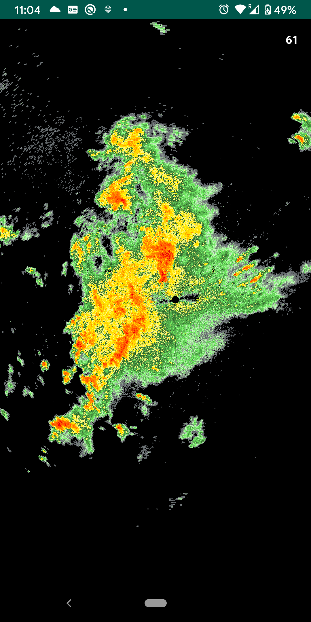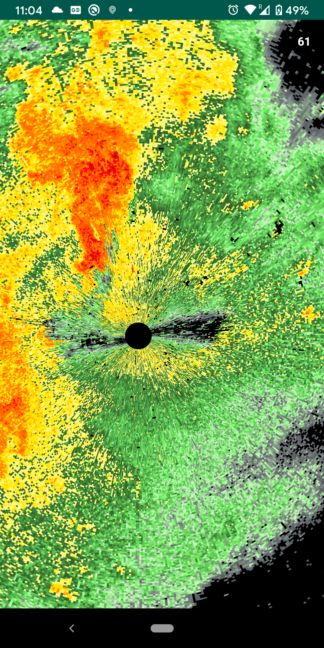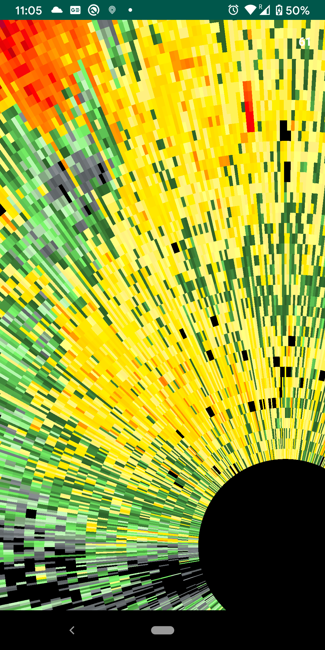NEXRAD Radars usually write data in NetCDF formats, however, understanding and parsing of NetCDF files are beyond the scope of this article series. For simplicity, I have collected relevant data in a JSON format file. Throughout this series, we will be working with such JSON file(s).

Here is miniaturized version of this JSON for reference

{
    "azimuth" : [ 94.0, 95.0],
    "gates" : [0.0, 999.0],
    "reflectivity" : [
        [22.5, 23.5],
        [23.5, 22.0]
    ]
}

You will see that there are three arrays in this file namely azimuth, gates, and reflectivity. Let’s try and understand what they mean.

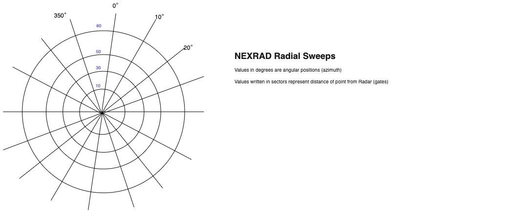
Consider the following image (sorry for my bad drawing!)

This image roughly represents how a NEXRAD Radar gathers data. As I previously stated that a NEXRAD Radar is a rotating antenna. It collects data in polar coordinates i.e. it gives us angles and distances from the center. Where center being position of Radar itself. Each concentric circle in the above image represents fixed distance from radar and each angle represents a data point at this fixed circle. Now coming back to our JSON azimuth is an array of these angles and gates is an array of distances from radar.

Third array that you see in JSON file is reflectivity value at each intersection point in above diagram. Reflectivity is essentially power of reflected signal which can tell us about level of precipitation in the atmosphere, structure of storm, potential of hail, boundaries of bad weather etc. For our purposes it will dictate the color of a pixel. Depending upon value of reflectivity at a given point we will fill color in our rendered image. If you look at sample JSON total number of points are 2 gates * 2 azimuth values and hence 4 reflectivity values. Each array within 2D reflectivity array represents values on one concentric circle.

In given JSON file we have 720 azimuth values and 1832 gates values. This mean that there are total of about 1.3 million (720 * 1862) polygons(trapezoids). In OpenGL polygons are rendered using triangle meshes. Although each polygon has some curve in the drawing but we can approximate it with trapezoids.

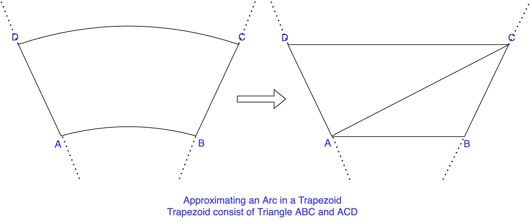
One trapezoid can be created using two triangles so total number of polygons that we need to draw comes out to be 2.6 million(2 * 1.3). Not to mention, each polygon has 3 vertices and each vertex has one color associated with it. This makes a total of 15.6 million data points that we need to work with. We will try and optimize this number in later parts of this series.

One more thing to note here is we have 4 different data points for any polygon. Now there are two things that can be done here.

1. First, we assign 4 different colors to 4 different points and interpolate those colors to fill the rest of the polygon. In OpenGL terms this is called SMOOTH_SHADING.
2. The second option is to fill the entire polygon with just one color and create a convention, for example, we can have lower-left corner data point representing entire polygon. This is similar(not exactly the same) to FLAT_SHADING in OpenGL.

While first option might seem like a more logical choice(also it looks better) it sometimes causes some information to get destroyed due to interpolation. Every data point is important here so usually the second approach is preferred.

In the next article lets try and implement the most basic version of this render using second approach.